GIT 2023 2024 Paper 2 Q2- Spreadsheet Question

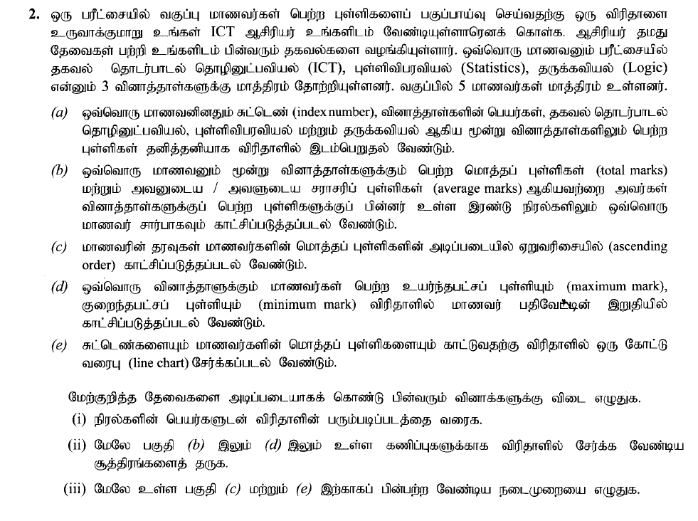
Assume that your ICT teacher has asked you to create a spreadsheet to analyze the marks obtained by the students in the class in an examination. The teacher has given you the following information about her requirements. Each student has sat for only 3 papers, namely ICT, Statistics, and Logic. The class has only 5 students.

• (a) The spreadsheet should contain the index number of the student, the names of the papers, the marks of papers ICT, Statistics, and Logic for each student separately.
• (b) The total marks scored by each student for all three papers and his/her average mark should be displayed for each student in the next two columns after the marks obtained for the papers.
• (c) The students’ data should be displayed in ascending order on the total marks of students.
• (d) The maximum mark and the minimum mark that students obtained for each paper should be displayed after the last student’s data in the spreadsheet.
• (e) A line chart should be included in the spreadsheet to show the index numbers and their total marks

Based on the above requirements, answer the following questions:

• (i) Draw a rough layout of the spreadsheet, giving the column names.
• (ii) Give the formulas to be included in the spreadsheet to compute the above (b) and (d) parts.
• (iii) Write down the procedures needed to be followed for the above parts (c) and (e)

• 

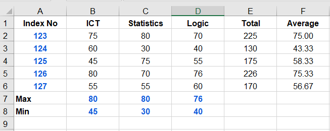
2(i) மாதிரி அமைப்பு: சுட்டெண், ICT, Statistics, Logic, மொத்தப்புள்ளி, சராசரி ஆகிய தலைப்புகளுடன் ஒரு அட்டவணையை உருவாக்க வேண்டும்.

2(ii) சூத்திரங்கள்

• மொத்தம்: =SUM(B2:D2)
• சராசரி: =AVERAGE(B2:D2)
• அதிகூடிய புள்ளி: =MAX(B2:B6)
• குறைந்த புள்ளி: =MIN(B2:B6)

2(iii) படிமுறைகள்:

• Sorting வரிசைப்படுத்தல்: தரவுகளைத் தெரிவு செய்து, Data > Sort என்பதற்குச் சென்று ‘Total Marks’ ஐ ‘Smallest to Largest’ எனத் தெரிவு செய்யவும்.
  
• வரைபடம்: சுட்டெண் மற்றும் மொத்தப்புள்ளி நிரல்களைத் தெரிவு செய்து, Insert > Line Chart என்பதை அழுத்தவும். (தேர்ந்தெடுக்கும்போது Ctrl ஐ அழுத்திப் பிடிக்கவும்),

2(ii) Formulas

• Total (b)
  =SUM(B2:D2)
• Average (b)
  =AVERAGE(B2:D2)
• Maximum (d)
  =MAX(B2:B6) (for ICT)
• Minimum (d)
  =MIN(B2:B6) (for ICT)

2(iii) Procedures:

• Sorting (c):
  Select all student data rows, go to the Data tab, click Sort, choose the Total column, and select Smallest to Largest (Ascending)
  
  Line Chart (e)
• Select the Index Number and Total columns simultaneously (hold Ctrl while selecting),
  Go to the Insert tab, and select Line Chart

Download Worksheet